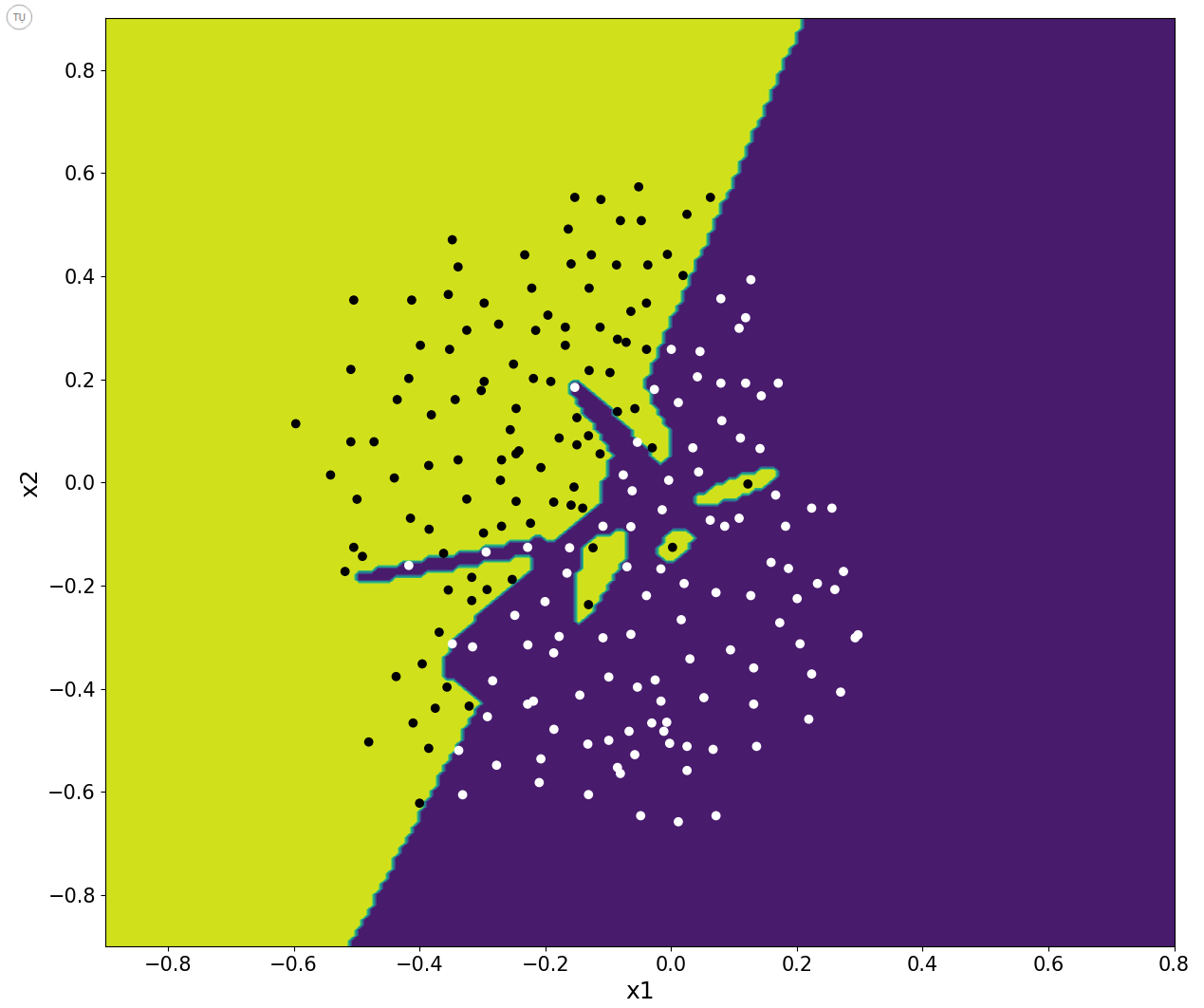
Dropout has been one of popular techniques to regularize Neural Networks in last couple of years. Before a discussion on probabilistic view of dropout, it is worth reviewing how dropout works. For the sake of discussion, I will use a toy example (shown in Figure-1), and a relatively small neural network. Size of network is 2x30x10x3x1 : A four layer network with an input layer, 3 hidden layers, and output layer ( Choice of this architecture was rather random ).

Figure-1 shows a trained model of neural network without using any regularization method. As seen, it is overfitting the data: Training accuracy is 100% while test accuracy is 92%. So, model does not generalize well. As a side note, yellow regions show locations, which model predicts to be where one class resides (black dots) while purple regions shows model’s predictions on where the other class resides (white dots). One way to improve the problem of overfitting data is to apply regularization such as dropout.

Figure-1

Review

So, what is dropout? Dropout is a method to sample sub-networks from a bigger network (as shown in Figure-2). It is a form of model averaging, where predictions of final trained network can be considered as averaging predictions of many smaller networks from a subset of a big network. It effectively reduces capacity of network, and prevents model from over-fitting the data.

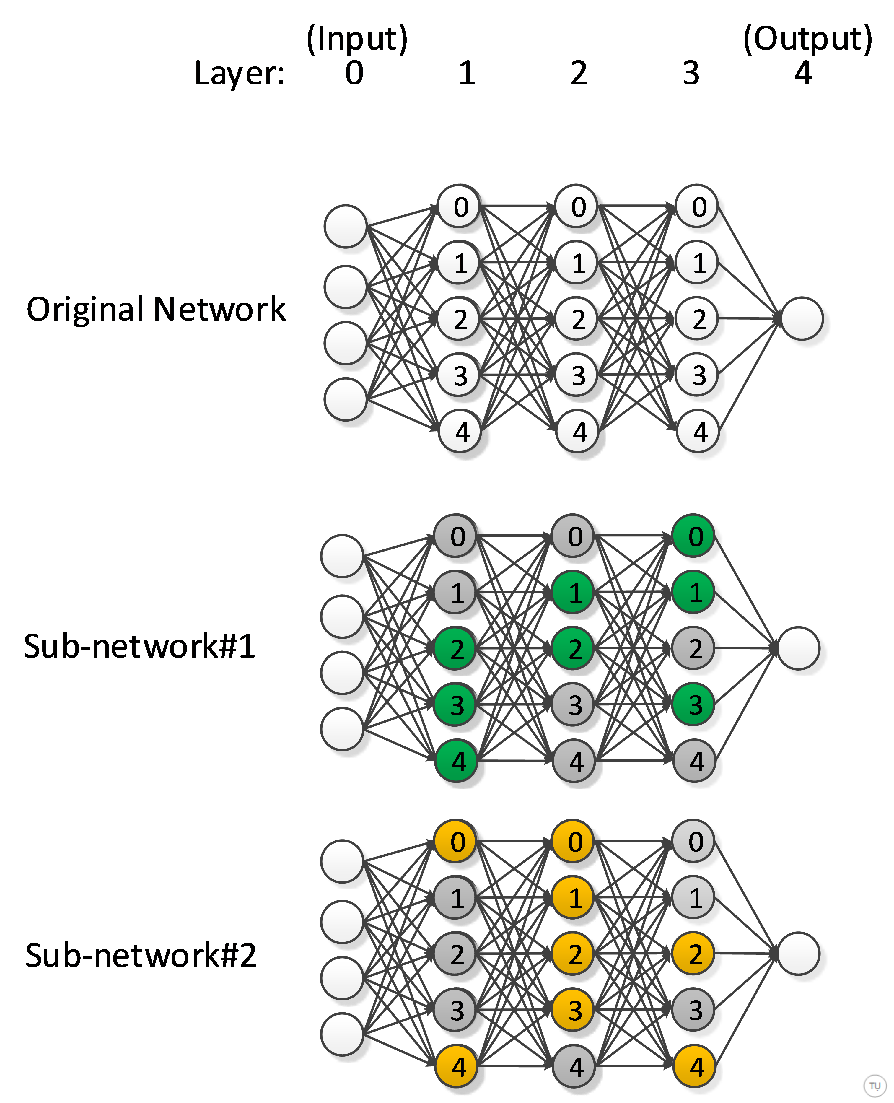
Figure-2

Once we decide on an initial architecture for our big network (say original network in Figure-2), there are two decisions to be made before we apply dropout to a neural network:

1. We need to decide on which layers of network we will apply dropout to? This can be modified later using a validation data set.
2. We need to choose a fixed retaining probability (p) for each layer selected in #1. Retaining probability is a hyperparameter, which, as in #1, can be tuned using a validation set later. But, for now, we can use 0.5 for p for each hidden layer selected in #1. Also, each layer can have a different probability. I will refer each of layers that we apply dropout to as dropout layer for brevity.

Once we make some initial decisions on #1 and #2, we can discuss what is going on during training and testing of the network:

Training:

Figure-3

As depicted in Figure-3 and Figure-4, for each forward pass during training, we sample a sub-network from bigger network (original network in Figure-2) by turning off some of the units in each dropout layer. For example, if retaining probability for layer l is p, then each unit within the layer can be retained with probability p (i.e. dropped out with probability (1-p)). The decision on which units to retain is random, and is independent of decisions on other units. Once a unit is dropped out, its incoming and outgoing connections will be inactive too. During back-propagation, we will only update the parameters of retained units and their connections.

In coding, this is achieved by applying a binary mask to the output of each dropout layer as shown in Figure-3. Elements of binary mask, [0, 1], are drawn independently from a Bernoulli distribution, and each has a probability p of being 1. Final output of dropout layer is result of element-wise multiplication of M*A, where M is the mask, and A is output of layer without mask.

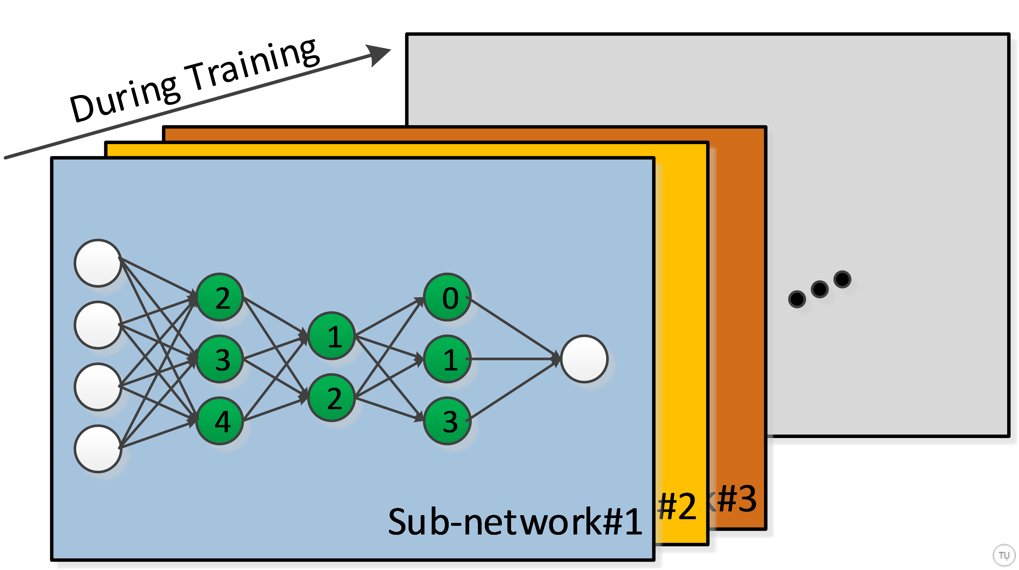
Figure-4

Testing:

During testing, dropout is turned off (i.e. there is no binary mask) so that we use our original big network with final weights learned during training (i.e. all units are active). Since we are using all units of network, we need to scale down output of each dropout layer by their respective probability p to keep output at test time same as expected output at training time. We can do this by scaling outgoing weights of dropout layer with p. This scaling of weights equates predictions of big network to average predictions of many sub-networks within big network.

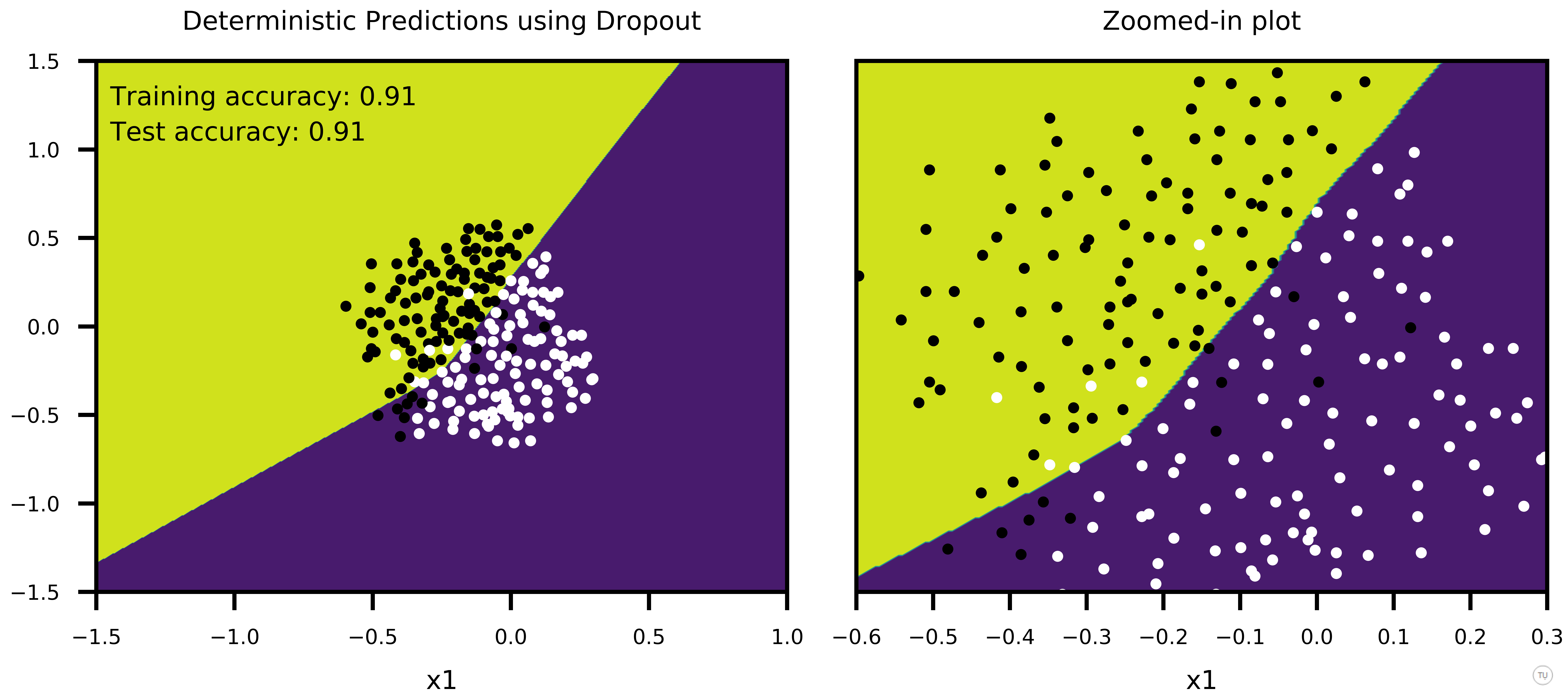
Figure-5

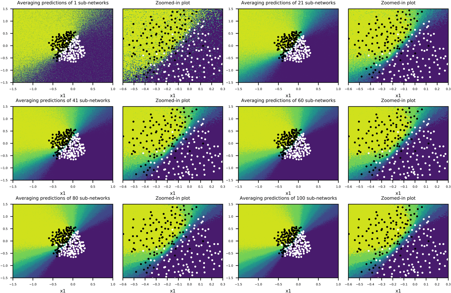
Figure-5 shows how predictions of big network using scaled weights (second row in the plot) compares to averaging predictions of many sub-networks sampled from the big network (first row in the plot). In this case, dropout is applied only on first two hidden layers with p=0.5 for both, and training is stopped pre-maturely (after 100 epochs). 100 sub-networks from big network are sampled, and their combined predictions as well as predictions of bigger network with scaled weights are plotted to show:

• Noisy outputs generated by sub-networks (First frame of GIF in first row of Figure-5, showing the predictions of a single sub-network)
• How average predictions of sub-networks evolve as more and more sub-networks are involved in predictions,
• How predictions of big network with scaled weights approximates averaging predictions of many smaller sub-networks (second row in Figure-5).

Thus, we can have a sense that scaling weights of bigger network is a good approximation to averaging predictions of many smaller sub-networks. Also note that both training and test accuracy is 91%, meaning that model can generalize well.

Figure-6 shows the case, where training is stopped after 1000 epochs. Predictions of each sub-network is less noisy, compared to Figure-5, and model accuracy is improved (Training Acc:95%, Test Acc: 94%). And again, big network with scaled weights shows a good approximation to averaging predictions of many sub-networks.

I should note that although weight-scaling is an approximation to geometric mean over all possible sub-networks, I used arithmetic mean to get average of sub-network predictions. Figure-5 and Figure-6 show that final decision boundaries of scaled network and averaged sub-networks are indeed very similar, and that arithmetic mean seems to give comparable results to geometric mean approximation.

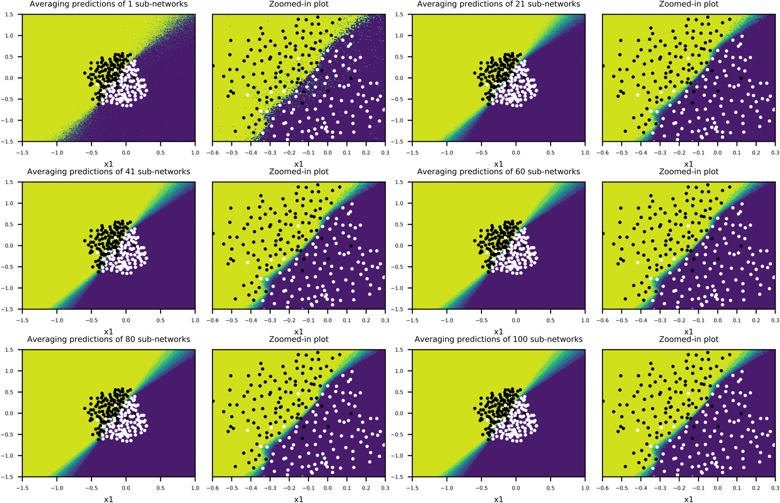
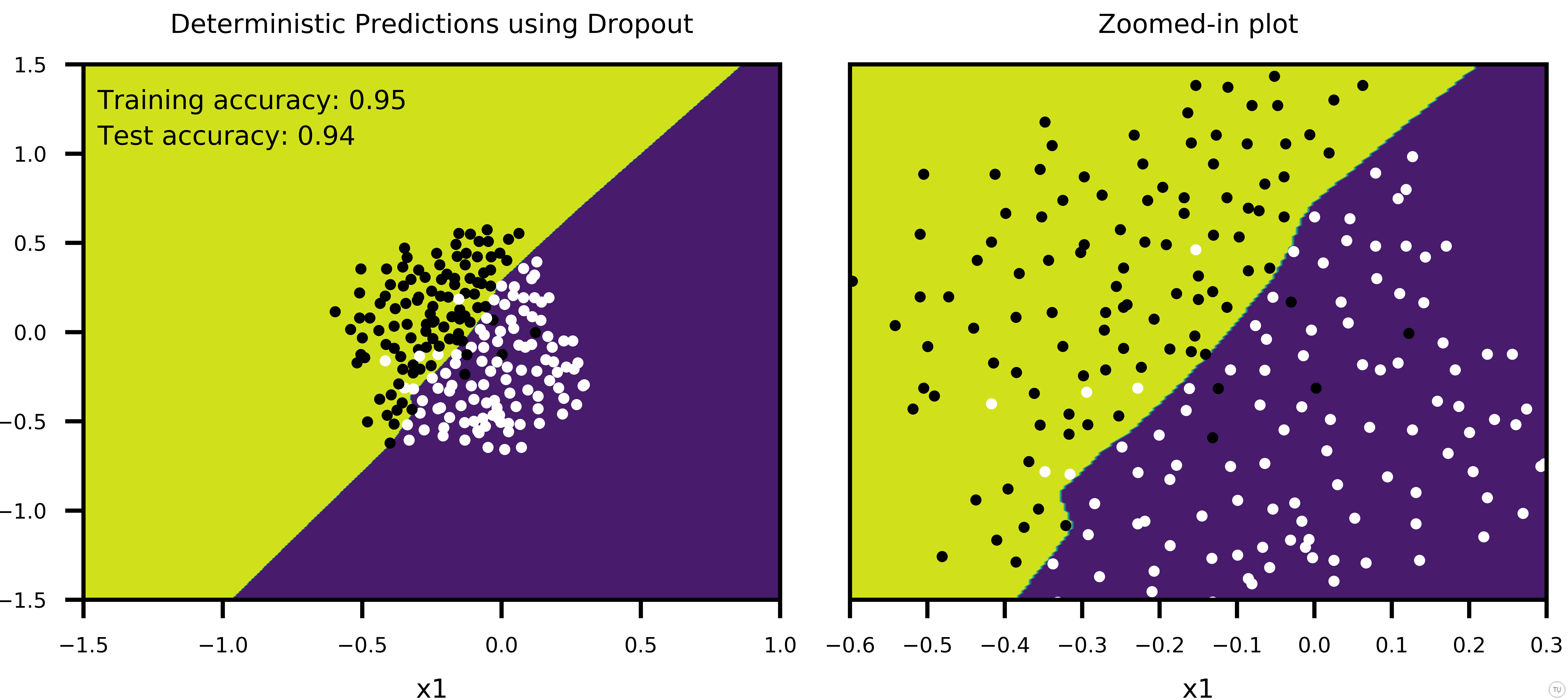
Figure-6

Now that we are done with how dropout works, we can move onto subject of this post.

Probabilistic View

Figure-7 shows the predictions of a single sub-network as well as predictions of big network with scaled-weights (same as Figure-6, only difference is that it shows predictions of a single sub-network, rather than a simulation using many sub-networks).

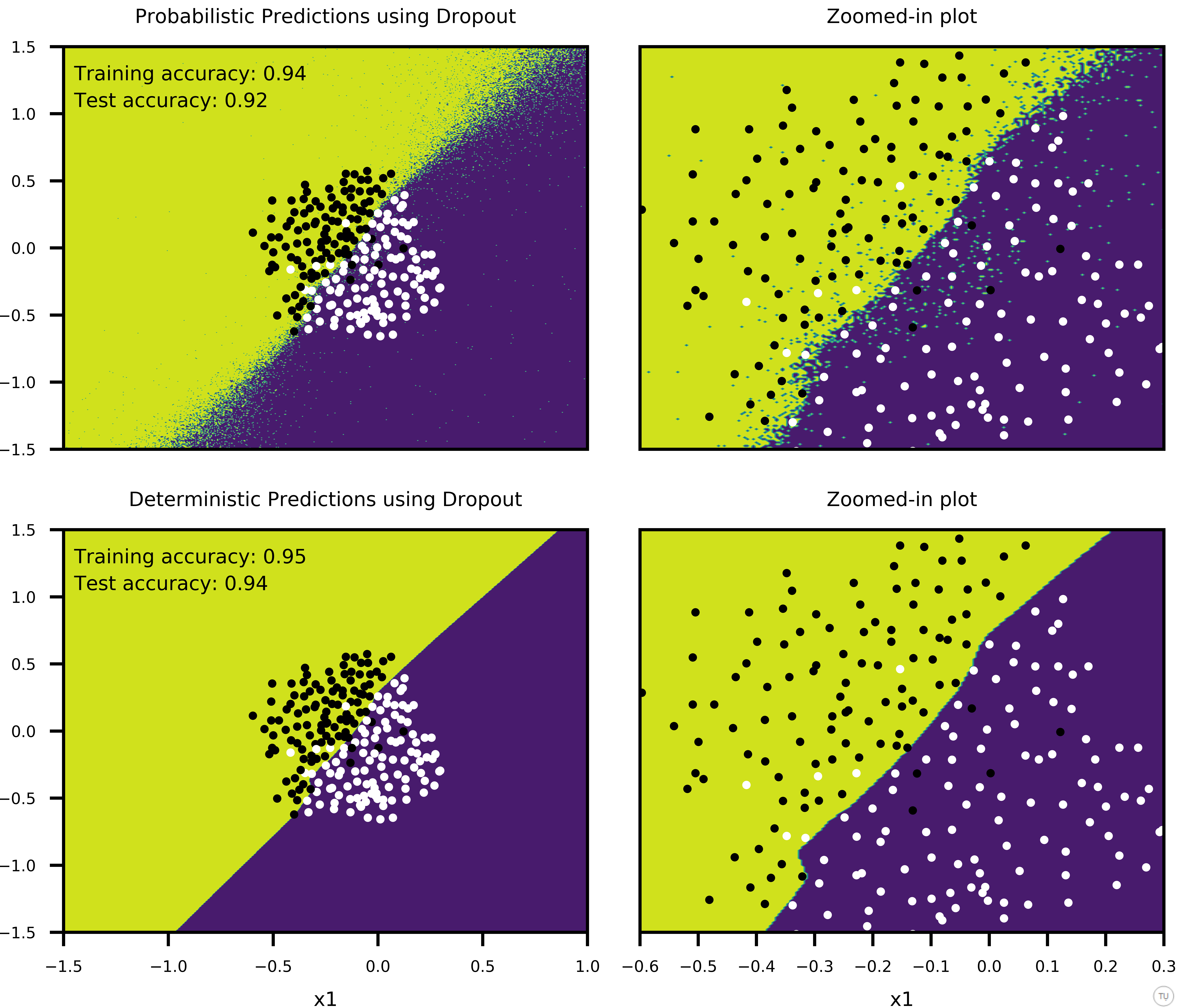
Figure-7

Difference between predictions of two networks ( a single sub-network vs big network with scaled weights) is following:

• Predictions of scaled network is deterministic, i.e. decision boundary is decisive. Everything on the left side of decision boundary is considered as one particular class whereas everything on the other side is predicted as another class. But, if you look at the data, only thing that we know is what is shown at the center of plot. We cannot say anything about four corner areas of plot since we have no data points there. We cannot even say much about decision boundary beyond center area of the plot either. So then the question is, how can we be so certain about a decision on those areas where we have no data point? We need a way to say how uncertain we are about our decisions.
• This is where the sub-network comes into play. Its predictions are noisy both along decision boundary as well as empty areas of plot where we have no data (See first frame of sub-network simulation in Figure-5, and Figure-6). Especially along the decision boundary, farther away we are from the data, more uncertain we are about our decisions. And noise generated by sub-network is not so random, in fact it is shaped by data. So noise distribution around a data point gives us an ability to see how uncertain we are about our decisions ‘in a particular region’, especially in places where we have no data (See evolution of decision boundary in regions where we have no data in Figure-6).

Lastly, it should be mentioned that predictions of scaled big network comes with probability information (this is also an approximation to averaging over many sub-networks), but noise distributions around a data point, or along the decision boundary provided by a sub-network is still insightful.

And for fun, Figure-8 shows a case where more data is added at one corner of plot to see how predictions of sub-networks evolve, compared to Figure-6 (everything else being equal).

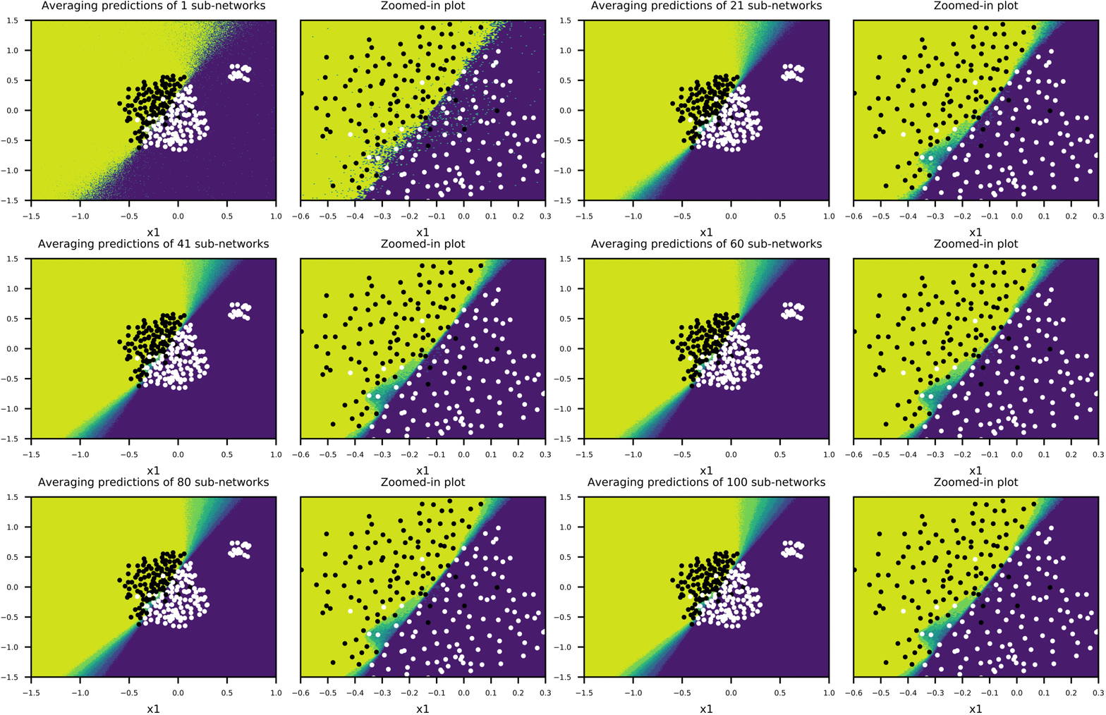
Figure-8

In summary, dropout is an interesting approach to regularization in that it gives way to probabilistic interpretation of data that can be utilized to state how certain we are about our predictions.

P.S.: It takes a lot of time and effort to prepare these diagrams / plots. So if you would like to re-use any of part of this post, I appreciate it if you add a reference to this blog.